MLinkPlanner 2.0 User Manual Part 2

MLinkPlanner 2.0

Point-to-Point and Point-to-Multipoint Microwave Link Planning Software

User Manual

Download in PDF format

Part 1

Part 2

Part 3

Part 4

Propagation Models for PtP and PtMP links

In this menu, user can select method which will be used to calculate microwave link performance as well as some parameters of this method.

Propagation Models

ITU-R P.530-17 Multipath Fading Model

Minimum value of the Flat Fade Margin, dB

Maximum value of the frequency diversity improvement factor for non-selective outage probability

Maximum value of the frequency diversity improvement factor for selective outage probability

Maximum value of the space diversity improvement factor for selective outage probability

Maximum value of the space and frequency diversity (four receivers) improvement factor for non-selective outage probability

Maximum value of the space and frequency diversity (four receivers) improvement factor for selective outage probability

Calculate selective fading

Ignore selective fading

Rec. ITU-R P. 453-9

Rec. ITU-R P. 453-14

Minimum allowable fade margin, dB
If fade margin is less than this value, calculation will be stopped (dashes will appear in report instead of calculated values).

Limiting the maximum value of the frequency diversity improvement factor for non-selective outage probability

Limiting the maximum value of the space diversity improvement factor for selective outage probability

Limiting the maximum value of the space and frequency diversity (four receivers) improvement factor for non-selective outage probability

Limiting the maximum value of the space and frequency diversity (four receivers) improvement factor for selective outage probability

Calculate selective fading

Ignore selective fading

Use Rec. ITU-R P. 453-9 refractive gradient data

Use Rec. ITU-R P. 453-14 refractive gradient data

Vigants-Barnett Multipath Fading Model

Minimum value of the Flat Fade Margin, dB

Minimum allowable fade margin, dB
If fade margin is less than this value, calculation will be stopped (dashes will appear in the report in place of calculated values).

Rain Attenuation

Rec. ITU-R P.530-17

Crane
- Select Crane 1996 rain region

None

Rain Attenuation Rain attenuation estimation according to Recommendation ITU-R P.530-17

Rain attenuation estimation according to Crane method, taking into account 1996 rain regions. To view rain regions for US and World, press I.

Do not calculate rain attenuation.

Gaseous Attenuation

Rec. ITU-R P.627-11

None

Calculate of gaseous attenuation according to recommendation ITU-R P.627-11

Do not calculate gaseous attenuation.

Diffraction

Rec. ITU-R P.526-15 (Complete Bullington method or Diffraction over multiple isolated cylinders method)

Deygout (the principle edge method with correction Rec. ITU-R P.526-11)

Epstein-Peterson

Calculation of diffraction attenuation by the Rec. ITU-R P.526-15 (complete Bullington method or Diffraction over multiple isolated cylinders method)

Calculation of diffraction attenuation by the Deygout (the principle edge method with correction Rec. ITU-R P.526-11)

Calculation of diffraction attenuation by the Epstein-Peterson method

Vegetation (according to Rec. ITU-R P.833-9)

A1 and Alfa parameters

Parameters A1 and Alfa for calculating attenuation in vegetation in accordance with ITU-T Rec. ITU-R P.833-9. Press i for information.

Planning Point-to-Point Links

Creating PtP Link

When sites have been created, you can create one or several microwave links. To start working with point-to-point links, open Point-to-Point item on main menu.

Point-to-Point main menu

First, it is necessary to include specification file of equipment family that is supposed to be involved in project.
Click on Add new product family button in Point-to-Point menu to include product family in your project. To download product family files from our website, click on Download product family files button and link will open in browser.

We are continually updating files with equipment parameters, but if such equipment is not on our website, then first create equipment specification file (see Equipment Editor).

Toolbar for PtP:

- Create a new PtP link.

- Select / Deselect all PtP links.

- Delete all selected PtP links.

- Summary report for all active PtP links in Microsoft Excel

Tx power general limits for all PtP links

not use

not use general limits

limit Tx power to max level, dBm

Maximum Tx power for transmitters of all PtP links in this project, dBm
From the general limit set in this menu and the limit set in a particular link, the most stringent limit is selected during calculation

limit EIRP to max level, dBm

Maximum EIRP for transmitters of all PtP links in this project, dBm
From the general limit set in this menu and the limit set in a particular link, the most stringent limit is selected during calculation

To create a PtP link, click on the Create a new PtP link button at the top of Point-to-Point menu, and the program will prompt you to select link ends, Site A and Site B, from sites created before. Then this link will appear in point-to-point tree and panel will open with its parameters. So that software can automatically calculate length of line consisting of several PtP links (necessary to distribute objectives by intervals - see Objectives section), choose link direction so it is easy to build line. For example, if there are sites A, B, C, D, E, then PtP links should be named as A-B, B-C, C-D, D-E (and not E-D, for example). Then when specifying beginning and end of line, for example A-E or B-D, the program will determine its topology and correctly take into account length of all PtP links in whole line. The same applies to branches of the main line.

PtP link parameters

PtP Link Toolbar:

- Create a new PtP link with the same parameters.

- Move this link up.

- Move this link down.

- Delete this link.

- Select / deselect all types of modulation and coding.

- Change the site A.

- Change the site B.

- Position the map with the link at the center of the screen.

- Generate the path profile for the link.

- Link report.

- Display the product specifications for the selected bandwidth in the form of a datasheet, which can be saved in PDF, Word, or Excel formats.

- Copy link parameters to the clipboard

- Paste link parameters from the clipboard

The required link can be selected from the list in the Point-to-Point menu or by double-clicking on it on the base map.

Path Profile

A path profile is a vertical sectional view of terrain created by plane passing through both ends of link. Path profile includes terrain elevation data, building and tree heights, and boundaries of water bodies.

MLinkPlanner creates path profiles using following GIS data:

Terrain elevation data 2-30 m plane resolution (Default DEM). For more details on data sources see Appendix 1 “Default DEM”. It is also possible to use custom DEM in GeoTIFF format with any plane resolution. To use custom DEM specify path to it in Settings menu and check corresponding box. File format requirements are outlined in Appendix 2 “Custom DEM Format”.
Global Tree Cover 1 arc sec (about 30 m) resolution data with information about tree heights. Data sources: High-Resolution Global Maps of 21st-Century Forest Cover Change Published by Hansen, Potapov, Moore, Hancher et al. Department of Geographical Sciences University of Maryland https://earthenginepartners.appspot.com and Jet Propulsion Laboratory California Institute of Technology https://landscape.jpl.nasa.gov/
Global 3D buildings data from OpenStreetMap project database. Data sources: Our buildings database which synchronizes with global OpenStreetMap (OSM) database.

All these types of geodata are downloaded for desired area automatically as needed; there is no need to worry about preloading geodata.

Creating the Path Profile with GIS

In created link click Generate path profile button. Warning dialog box will appear indicating that path profile data will be changed. You should specify average building floor height (typically 3 m) in this window. OSM project database usually contains information about number of floors of buildings rather than their height in meters. Building height in the path profile will usually be based on the number of floors and floor height. You will also have to specify the height of the buildings for which the OSM project database does not have information. Such buildings will be highlighted in red in the path profile.
If a building affects the qualitative characteristics of the path profile as a critical obstruction, check the building’s height with third-party sources to verify its exact height. The user can override the forest height information obtained from the Global Forest Change records and set a new value to be used in a path profile

Path Profile Creating Settings

Click OK, and after a couple of seconds, the information about terrain elevation and clutter characteristics along the path profile will appear in the table cells. The view of the path profile will be displayed in the top right panel.

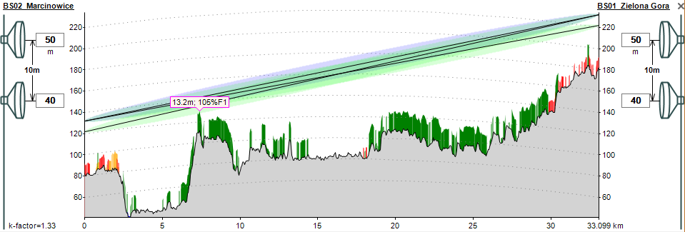
Path Profile

Clutter:

Green: trees

Orange: buildings whose height or number of floors can be found in the OpenStreetMap database
Red: buildings whose height and number of floors are missing in the OpenStreetMap database

Editing the Path Profile

Terrain elevations can be edited manually in the corresponding cells of the elevation table. To edit terrain elevations for multiple cells, select the required cells and enter a new value. The new elevation will be saved to all selected cells, and the information about old elevations will be automatically removed. Only end values of this range will remain. To delete an entire row in the table, click on the triangle icon at the beginning of the row to select either a single row or multiple rows (by dragging the mouse or holding the Shift key and using the up or down arrow keys) and press Delete.

If you highlight a segment on the path profile by clicking and dragging with the left mouse button, that segment will also be highlighted in the terrain elevation table, clutter table, and on the base map. Likewise, if you select rows in either elevation or clutter table, it will highlight the corresponding section in both path profile view and on base map.

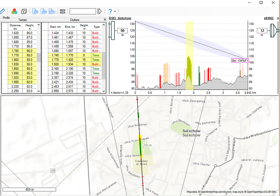
Highlighting the path profile segment

The clutter can also be edited manually in corresponding cells of clutter table. To delete an entire row in table, click on triangle icon at beginning of row to select either single row or multiple rows (by dragging mouse or holding Shift key and using up or down arrow keys) and press Delete.

Creating the Path Profile Manually

The application allows you to create a path profile by manually specifying all elevations on path profile.
Information about forests, buildings, and water bodies can be entered based on base maps which you can open right within application. Many online services allow you to view cartographic materials. They all differ in such parameters as map scale, coverage, and displayed objects. Depending on specific area where link is located, you may find one or several services useful. It is also important to select proper scale of map. More information about using custom base maps can be found within application.

After analyzing basemap along line of path profile, you can enter boundaries of forests, buildings, and water bodies. To do that, on base map right-click on point on link path where you want to enter start of clutter object segment. A context menu will open where you can select corresponding types of segment. When ends of segment are marked, number field will appear that you must fill in to indicate forest or building height. On path profile forest is highlighted green, building orange, and water area blue. Table entries for clutter and water information will be created automatically. You can delete any segment by right-clicking on it and selecting corresponding action in context menu that appears.

Start a Building Segment

Start a Tree Segment

Start a Water Segment

End Segment

Delete the Nearest Segment

Move Site A

Move Site B

Specify the beginning of the building segment on the path profile.

Specify the beginning of the tree segment on the path profile.

Specify the beginning of the water segment on the path profile.

Specify the end of any segment.

Delete any nearest segment.

Move site A to the specified location.

Move site B to the specified location.

The following must be observed when creating a path profile manually:
1. The first elevation point must have a zero distance.
2. The path profile must have at least two points.
3. A clutter object must not extend beyond the last terrain point.

For more information about creating a path profile for microwave links, visit our
YouTube channel.

Entering Parameters of PtP Links

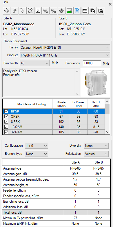
In the drop-down lists, select the product family from those previously connected to the project, then select the equipment model (product), channel bandwidth, and frequency band. After that, general information about the selected equipment, its image, channel bitrates, and basic energy parameters for each type of modulation supported by the equipment will appear below.

Below is a description of all input parameters that may be necessary to specify. The required input parameters are determined by the application automatically based on the equipment configuration and calculation requirements.

Frequency, MHz

Configuration

Diversity

Branching Type

Polarization

Frequency Spacing, MHz

Mean frequency of the microwave link, MHz

The number of working and reserve trunks

Diversity configurations (None, Space Diversity, Frequency Diversity, Comb-4Rx)

Hot Standby (HSB) /XPIC (Cochannel)/HSB+XPIC/MIMO 2x2

Polarization type (Vertical or Horizontal)

The frequency spacing between TX channels for frequency diversity. Required if frequency or combined diversity is selected.

Antenna, feeder, and branching parameters for the Main and Diversity paths (when using space diversity):

Antenna Type

Antenna Gain, dBi

Vertical Antenna Beam Width, Degrees

Antenna model; information only

Antenna gain, dBi

Antenna 3 dB beam width in a vertical plane; use only for reflection analysis. The default value is 3 degrees.

Antenna Height, m

Antenna installation height relative to ground level, m.
You can also change the antenna height in the profile window.

Feeder Length, m

Feeder Specific Loss, dB/m

Branching Loss, dB

Additional Loss, dB

Total loss, dB

Maximum Tx power limit, dBm

Maximum EIRP limit, dBm

Feeder length to the primary antenna; the default value is 0 m.

Feeder specific loss; default value is 0 dB/m.

Branching loss at Tx and Rx (if any); the default value is 0 dB.

Additional loss; default value is 0 dB.

Total loss, dB. The calculated value.

Maximum Tx power for transmitters of this link, dBm
From the general limit that is set in the PtP menu and the limit that is set in a particular link, the most stringent limit is selected during calculation. To remove the maximum limit, highlight the value and press the Delete key; then “None” will appear.

Maximum EIRP for transmitters of this link, dBm
From the general limit that is set in the PtP menu and the limit that is set in a particular link, the most stringent limit is selected during calculation. To remove the maximum limit, highlight the value and press the Delete key; then “None” will appear.

PtP Link Error Performance and Availability Prediction

To do the link performance prediction, click the Report button. The calculation will be performed only for those types of modulation that are marked as active in table.

You can switch between short report view and full report view. Short report displays only calculation results while full report displays input parameters, calculation results, path profile drawing and path profile diagram on map.

You can print report or save it as PDF, Microsoft Word or Excel.

Full PtP Link Report

You can also save summary information for all Point-to-Point links in an Excel spreadsheet by clicking on “Summary Report” button on Point-to-Point main menu.

Microsoft Excel Summary Report for Point-to-Point links

Objectives

The objectives for PtP links are set in Point-to-Point main menu item. Here you need to specify your approach to determining reliability of microwave link and if necessary, enter additional link parameters to calculate performance and availability objectives.

Objectives

Total Annual Time Below Level

Total Annual Time Below Level refers to the total amount of time in a year that the signal level falls below a certain threshold. Outage times are reported for the worst month and annually without considering the fade duration. The annual rain outage is simply added to the annual multipath outage for the total annual outage. This assumes that the conditions for high-intensity rain and severe multipath fading are different and the two fading mechanisms do not occur at the same time. Outage probabilities can be expressed as availability (e.g., 99.95%) or unavailability (in seconds).

Use of Error Performance Objectives (ITU-R F.1668) and Availability Objectives (ITU-R F.1703)

Error Performance Objectives (ITU-R F.1668) and Availability Objectives (ITU-R F.1703) are used to calculate Severely Errored Seconds for the worst month as a ratio (SESR) and in seconds (SES). Availability is reported as a ratio per year, while unavailability is reported in seconds per year. It is assumed that a rain fade will always last longer than 10 consecutive seconds, and therefore, the rain outage is always classed as unavailability.

For the objectives calculation, you have to specify if the link is part of an International or National Link and select among the relevant subcategories—Long Haul, Short Haul, Access. If the line consists of several links, for the distribution of the objective in accordance with the ratio of the length of the link to the total length of the line, specify the first and last sites of the line. The program will calculate the total length of the line, taking into account its topology, and when calculating the objective, will be distributed among the links in proportion to their length

Optimizing Antenna Heights

MLinkPlanner can calculate the height of main and diversity antennas using different clearance criteria.
To calculate antenna heights, select the desired link, then click the Optimizing Antenna Heights icon on the top toolbar.

The general procedure for determining the minimum required antenna heights on a link is to verify the required clearance of the first Fresnel zone for various expected values of the ratio of the equivalent Earth radius to the real radius (k-factor). Different methods have different requirements for clearance and k-factor value.

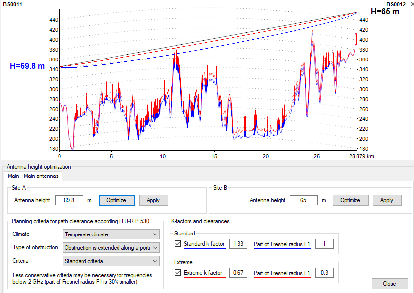
Antenna height optimization panel

Optimizing Antenna Heights According to Rec. ITU-R P.530-17

Climate

Temperate climate / Tropical climate

Type of Obstruction

Obstruction is extended along a portion of the path / Single isolated path obstruction

Criteria

Standard / Less conservative criteria. It may be necessary for frequencies less than about 2 GHz to avoid unacceptably large antenna heights.

Standard k-factor

The median value of the k-factor (equivalent Earth radius factor) for standard atmosphere. Can be modified by the designer.

Extreme k-factor

The lowest expected (minimum) value of the k-factor, computed from ITU-R Rec. P.530-17, as a function of path length. Can be modified by the designer.

Part of Fresnel Radius

Part of the First Fresnel ellipsoid that is required to be free of any obstruction for the appropriate value of the k-factor. Is automatically determined depending on the Type of Climate, Type of the Obstruction, and Criteria from above, but can be modified by the designer.

In a space diversity configuration, the minimum heights of secondary antennas are calculated without taking into account climate and extreme k-factor, as per Rec. ITU-R P.530-17. Minimum antenna height is calculated with consideration for clutter (forest and buildings) located on the path profile.
Once the required preferences are selected, click “Optimize” and the minimum antenna height will appear on the left. The height of the response antenna will be fixed at the current value. The path profile image will display the criterion used to calculate the antenna height. Click “Apply” to change the antenna height according to the calculated value. To discard the calculated value, click “Cancel.”

Path profile showing a triggered criterion

Reflection Analysis

Reflection Analysis allows the user to identify possible specular reflection points on the link path profile and evaluate the application of various specular reflection reduction methods.

To open the Reflection Analysis window, click the Reflection analysis button on the main window. The left-hand part of the panel will be disabled; to exit this mode, use the main menu.

k-factor

k-factor, for which the reflection points are searched
It is recommended that reflection points be determined for large k-factor values (at least 10).

Polarization

Vertical /Horizontal

To reduce the effect of the reflected wave, it is recommended to select vertical polarization.

Reflecting Surface Type

Sea water
Fresh water
Wet ground
Very dry ground
Ice
The type of surface from which the reflection occurs. Each of the above surface types have their own values of Relative dielectric constant and Electrical conductivity.

Relative Dielectric Constant

Relative dielectric constant is a dimensionless parameter. It’s automatically determined depending on the Reflecting surface type from above, but can be modified by the designer.

Electrical Conductivity

Electrical conductivity [ohm‐1 m‐1]. It’s automatically determined depending on the Reflecting surface type from above, but can be modified by the designer.

Consider Clutter on the Reflected Paths

If this check-box is active, then when the incident or reflected rays intersect with ground obstacles (forest or trees), these rays will be screened.

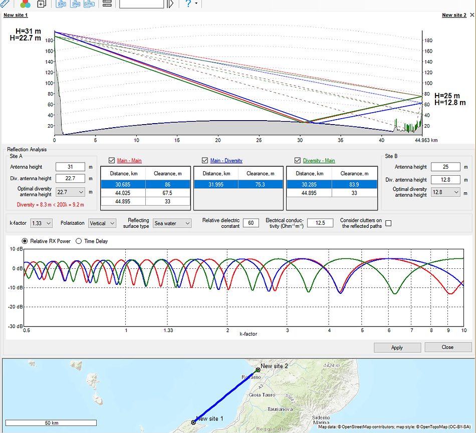
The path profile will display all possible direct and ground-reflected rays for the Main-Main paths and, in a space diversity configuration, for the Main-Diversity and Diversity-Main paths. The table below will show the distances to and clearance at each of the reflection points.

You can view Relative Rx Power vs. k-factor chart for any reflection point and any of the Main-Main, Main-Diversity, or Diversity-Main paths by clicking on the desired point in the table. Note that you need to specify the beam width for each of the antennas in Site A and Site B to calculate Relative Rx Power vs. k-factor chart.

In addition to Relative Rx Power vs. k-factor, you can also display Time Delay vs. k-factor chart. On this plot, the relative signal delay in nanoseconds between direct and reflected signal is displayed for each of Main-Main, Main-Diversity or Diversity-Main paths. If reflected signal delay is greater than 10-20 nanoseconds, performance problems on high-capacity systems can occur.

Reflection analysis

Estimation of Specular Reflection Reduction without Using Space Diversity

If there is specular reflection along path and you are not going to use space diversity, application can estimate effectiveness of following methods for reducing effect of reflected ray on resulting signal for systems without space diversity recommended in Rec. ITU-R P.530-17:

Increase of path inclination
Shielding of reflection point
Moving of reflection point to poorer reflecting surface
Reduction of path clearance
Choice of vertical polarization

In most cases, these methods (except for last one) are limited to selecting primary antenna height on right or left

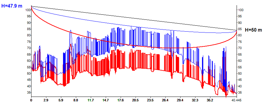
Estimation of Specular Reflection Effect with Space Diversity

The most efficient way to eliminate effect of specular reflection is to use space diversity techniques. The most often used technique is vertical space diversity. MLinkPlanner allows you to determine receive antenna heights with enough spacing to maintain uncorrelated direct and reflected signal so that when received signal level for primary antenna is zero (in fade), signal is near peak for diversity antenna and vice versa. Right-hand part of window displays heights of diversity antennas determined based on optimum antenna spacing as per Rec. ITU-R P.530-17 i.e., case when received signal levels at primary and secondary antennas must display maximum difference (maximum and minimum) across full range of k-factor to minimize effect of specular reflection on received signal level.

To estimate the effect of space diversity, perform the following steps:

Select a space diversity configuration for both Site A and Site B.
Select a reflection point for each path using the mouse button.
Select one of the optimum heights of the secondary antenna from the series in the right section of the window using the mouse button.

You will then be able to view the received signal level for each antenna on the chart. By changing the antenna height, you can see how the received signal level will change.

In a space diversity configuration, if the vertical spacing between antennas is less than 200 times the wavelength (which is a common rule for reducing the effect of multipath propagation on performance indicators), a warning will appear next to the spacing on the profile and its value in meters (i.e., 200 times the wavelength) will be displayed.

To determine heights of primary and secondary antennas in a space diversity configuration, the following conditions must be met:

The maximum difference between received signal levels of primary and secondary antennas must be observed across full range of k-factor to eliminate effect of specular reflection (if any).
Primary and secondary antennas must be at least 200 times wavelength to eliminate effect of multipath propagation.
Primary and secondary antennas must satisfy clearance criteria described in Rec. ITU-R P.530-17.